Mayavi2

The Simphony-Mayavi library provides a plugin for Mayavi2 to easily create mayavi Source instances from SimPhoNy CUDS datasets and files.

Any CUDS datastet can be adapted as a mayavi Source using CUDSSource. If CUDS datasets are to be loaded from a CUDS native file, it maybe easier to use CUDSFileSource which does the loading for you. Similarly, if the CUDS datasets are from a SimPhoNy engine wrapper, EngineSource may be used. All of these Source objects provide an update function that allows the user to refresh visualisation once the CUDS dataset is modified.

With the provided tools one can use the SimPhoNy libraries to work inside the Mayavi2 application, as it is demonstrated in the examples.

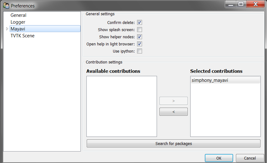
Open CUDS Files in Mayavi2

In order for mayavi2 to understand *.cuds files one needs to make sure that the simpony_mayavi plugin has been selected and activated in the Mayavi2 preferences dialog.

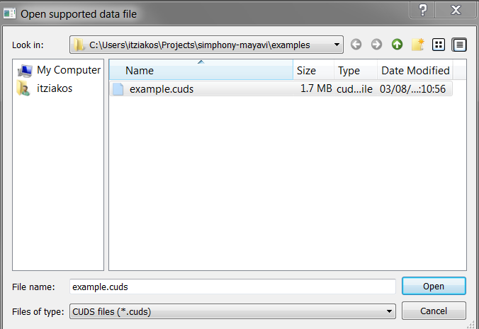
Cuds files are supported in the Open File.. dialog. After running the provided example, load the example.cuds file into Mayavi2.

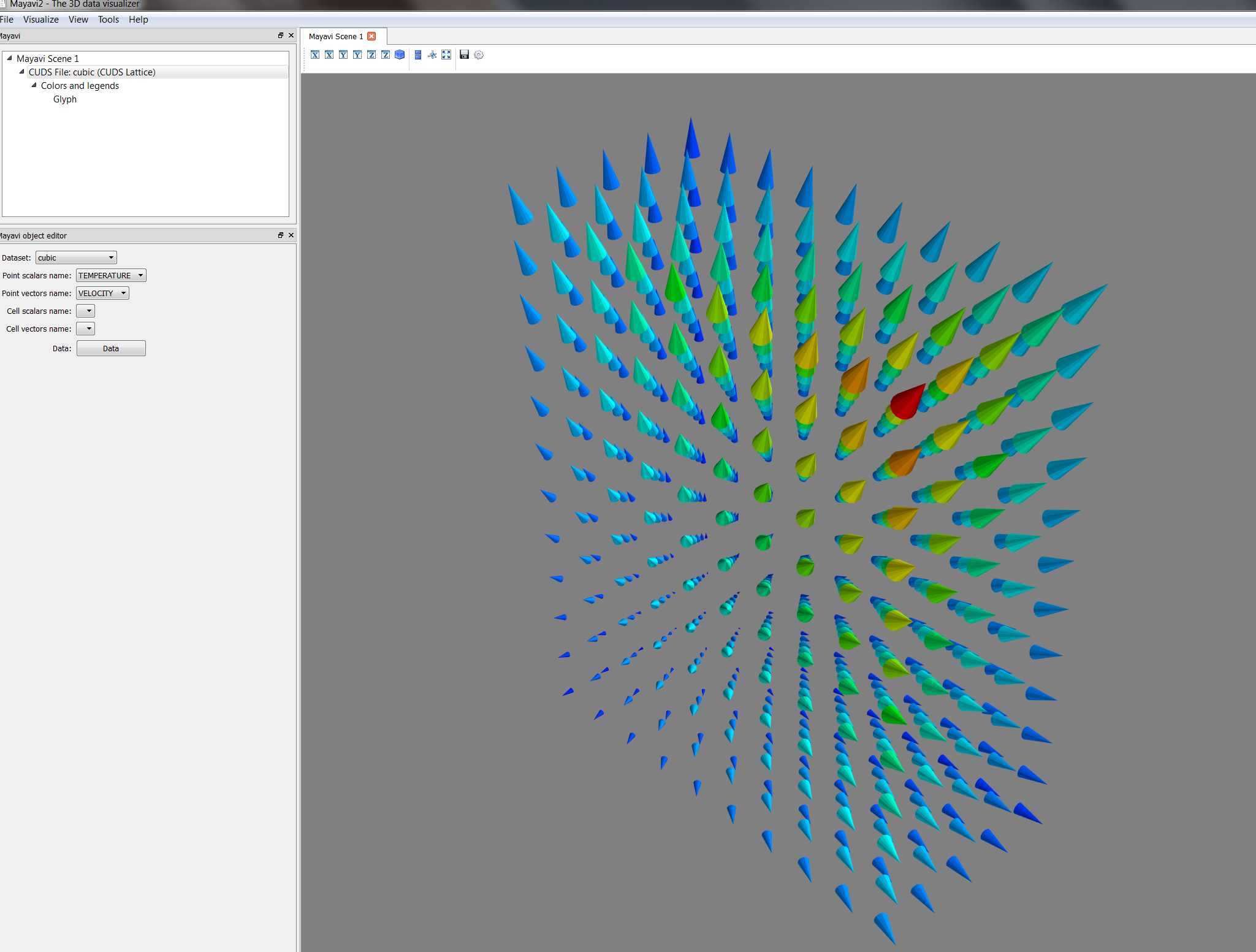
When loaded a CUDSFile is converted into a Mayavi Source and the user can add normal Mayavi modules to visualise the currently selected CUDS container from the available containers in the file.

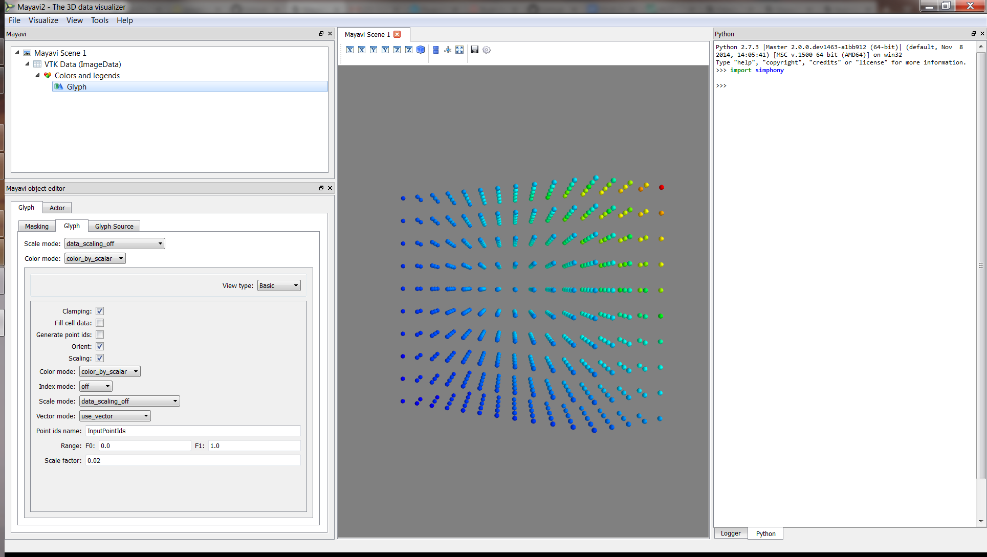
In the example we load the container named cubic and attach the Glyph module to draw a cone at each point to visualise TEMPERATURE and VELOCITY in the Mayavi Scene.

View CUDS in Mayavi2

Source from a CUDS Mesh

from numpy import array
from mayavi.scripts import mayavi2

from simphony.cuds.mesh import Mesh, Point, Cell, Edge, Face
from simphony.core.data_container import DataContainer


points = array([
    [0, 0, 0], [1, 0, 0], [0, 1, 0], [0, 0, 1],
    [2, 0, 0], [3, 0, 0], [3, 1, 0], [2, 1, 0],
    [2, 0, 1], [3, 0, 1], [3, 1, 1], [2, 1, 1]],
    'f')

cells = [
    [0, 1, 2, 3],  # tetra
    [4, 5, 6, 7, 8, 9, 10, 11]]  # hex

faces = [[2, 7, 11]]
edges = [[1, 4], [3, 8]]

container = Mesh('test')

# add points
point_iter = (Point(coordinates=point, data=DataContainer(TEMPERATURE=index))
              for index, point in enumerate(points))
uids = container.add(point_iter)

# add edges
edge_iter = (Edge(points=[uids[index] for index in element],
                  data=DataContainer(TEMPERATURE=index + 20))
             for index, element in enumerate(edges))
edge_uids = container.add(edge_iter)

# add faces
face_iter = (Face(points=[uids[index] for index in element],
                  data=DataContainer(TEMPERATURE=index + 30))
             for index, element in enumerate(faces))
face_uids = container.add(face_iter)

# add cells
cell_iter = (Cell(points=[uids[index] for index in element],
                  data=DataContainer(TEMPERATURE=index + 40))
             for index, element in enumerate(cells))
cell_uids = container.add(cell_iter)


# Now view the data.
@mayavi2.standalone
def view():
    from mayavi.modules.surface import Surface
    from simphony_mayavi.sources.api import CUDSSource

    mayavi.new_scene()  # noqa
    src = CUDSSource(cuds=container)
    mayavi.add_source(src)  # noqa
    s = Surface()
    mayavi.add_module(s)  # noqa

if __name__ == '__main__':
    view()

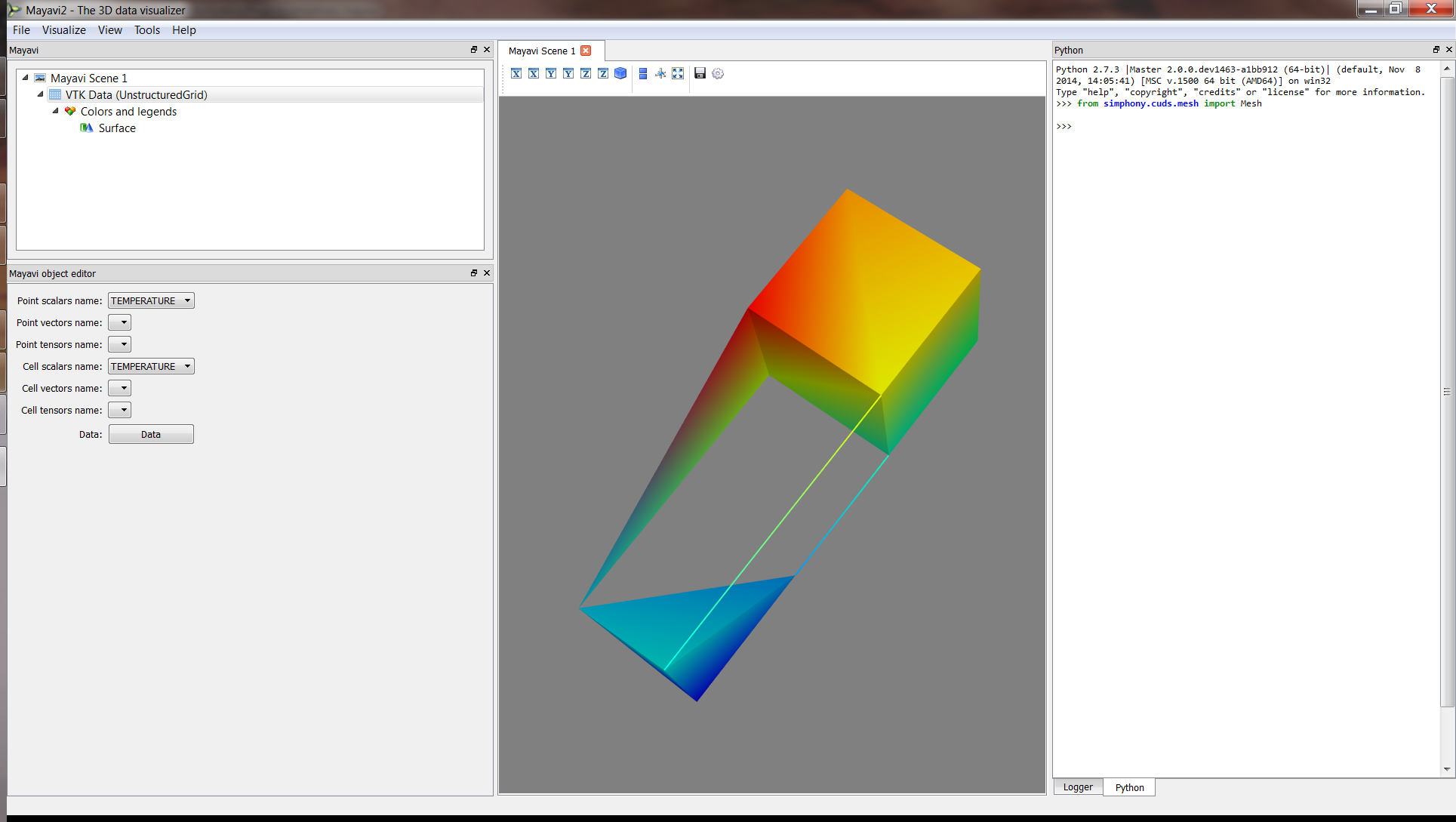
Use the provided example to create a CUDS Mesh and visualise directly in Mayavi2.

Source from a CUDS Lattice

import numpy

from mayavi.scripts import mayavi2
from simphony.cuds.lattice import make_cubic_lattice
from simphony.core.cuba import CUBA

cubic = make_cubic_lattice("cubic", 0.1, (5, 10, 12))


def add_temperature(lattice):
    new_nodes = []
    for node in lattice.iter(item_type=CUBA.NODE):
        index = numpy.array(node.index) + 1.0
        node.data[CUBA.TEMPERATURE] = numpy.prod(index)
        new_nodes.append(node)
    lattice.update(new_nodes)

add_temperature(cubic)


# Now view the data.
@mayavi2.standalone
def view(lattice):
    from mayavi.modules.glyph import Glyph
    from simphony_mayavi.sources.api import CUDSSource
    mayavi.new_scene()  # noqa
    src = CUDSSource(cuds=lattice)
    mayavi.add_source(src)  # noqa
    g = Glyph()
    gs = g.glyph.glyph_source
    gs.glyph_source = gs.glyph_dict['sphere_source']
    g.glyph.glyph.scale_factor = 0.02
    g.glyph.scale_mode = 'data_scaling_off'
    mayavi.add_module(g)  # noqa

if __name__ == '__main__':
    view(cubic)

Use the provided example to create a CUDS Lattice and visualise directly in Mayavi2.

Source for a CUDS Particles

from numpy import array
from mayavi.scripts import mayavi2

from simphony.cuds.particles import Particles, Particle, Bond
from simphony.core.data_container import DataContainer

points = array([[0, 0, 0], [1, 0, 0], [0, 1, 0], [0, 0, 1]], 'f')
bonds = array([[0, 1], [0, 3], [1, 3, 2]])
temperature = array([10., 20., 30., 40.])

container = Particles('test')

# add particles
particle_iter = (Particle(coordinates=point,
                          data=DataContainer(TEMPERATURE=temperature[index]))
                 for index, point in enumerate(points))
uids = container.add(particle_iter)

# add bonds
bond_iter = (Bond(particles=[uids[index] for index in indices])
             for indices in bonds)
container.add(bond_iter)


# Now view the data.
@mayavi2.standalone
def view():
    from mayavi.modules.surface import Surface
    from mayavi.modules.glyph import Glyph
    from simphony_mayavi.sources.api import CUDSSource

    mayavi.new_scene()  # noqa
    src = CUDSSource(cuds=container)
    mayavi.add_source(src)  # noqa
    g = Glyph()
    gs = g.glyph.glyph_source
    gs.glyph_source = gs.glyph_dict['sphere_source']
    g.glyph.glyph.scale_factor = 0.05
    g.glyph.scale_mode = 'data_scaling_off'
    s = Surface()
    s.actor.mapper.scalar_visibility = False

    mayavi.add_module(g)  # noqa
    mayavi.add_module(s)  # noqa

if __name__ == '__main__':
    view()

Use the provided example to create a CUDS Particles and visualise directly in Mayavi2.

Source from a CUDS native file

from contextlib import closing

import numpy
from mayavi.scripts import mayavi2

from simphony.core.cuba import CUBA
from simphony.cuds.lattice import (make_hexagonal_lattice,
                                   make_orthorhombic_lattice)
from simphony.io.h5_cuds import H5CUDS

# create some datasets to be saved in a file
hexagonal = make_hexagonal_lattice(
    'hexagonal', 0.1, 0.1, (5, 5, 5), (5, 4, 0))

orthorhombic = make_orthorhombic_lattice(
    'orthorhombic', (0.1, 0.2, 0.3), (5, 5, 5), (5, 4, 0))


def add_temperature(lattice):
    new_nodes = []
    for node in lattice.iter(item_type=CUBA.NODE):
        index = numpy.array(node.index) + 1.0
        node.data[CUBA.TEMPERATURE] = numpy.prod(index)
        new_nodes.append(node)
    lattice.update(new_nodes)

# add some scalar data (i.e. temperature)
add_temperature(hexagonal)
add_temperature(orthorhombic)

# save the data into cuds.
with closing(H5CUDS.open('lattices.cuds', 'w')) as handle:
    handle.add_dataset(hexagonal)
    handle.add_dataset(orthorhombic)


@mayavi2.standalone
def view():
    from mayavi import mlab
    from mayavi.modules.glyph import Glyph
    from simphony_mayavi.sources.api import CUDSFileSource

    mayavi.new_scene()

    # Mayavi Source
    src = CUDSFileSource()
    src.initialize('lattices.cuds')

    # choose a dataset for display
    src.dataset = 'orthorhombic'

    mayavi.add_source(src)

    # customise the visualisation
    g = Glyph()
    gs = g.glyph.glyph_source
    gs.glyph_source = gs.glyph_dict['sphere_source']
    g.glyph.glyph.scale_factor = 0.05
    g.glyph.scale_mode = 'data_scaling_off'
    mayavi.add_module(g)

    # add legend
    module_manager = src.children[0]
    module_manager.scalar_lut_manager.show_scalar_bar = True
    module_manager.scalar_lut_manager.show_legend = True

    # customise the camera
    mlab.view(63., 38., 3., [5., 4., 0.])


if __name__ == '__main__':
    view()

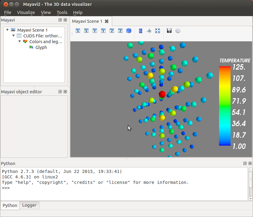
Use the provided example to load data from a CUDS file and visualise directly in Mayavi2.

Source from a SimPhoNy engine wrapper

from mayavi.scripts import mayavi2
from simphony_mayavi.tests.testing_utils import DummyEngine

# Comply to SimPhoNy modeling engine API
engine_wrapper = DummyEngine()


@mayavi2.standalone
def view():
    from mayavi.modules.glyph import Glyph
    from simphony_mayavi.sources.api import EngineSource
    from mayavi import mlab

    # Define EngineSource, choose dataset
    src = EngineSource(engine=engine_wrapper,
                       dataset="particles")

    # choose the CUBA attribute for display
    src.point_scalars_name = "TEMPERATURE"

    mayavi.add_source(src)

    # customise the visualisation
    g = Glyph()
    gs = g.glyph.glyph_source
    gs.glyph_source = gs.glyph_dict['sphere_source']
    g.glyph.glyph.scale_factor = 0.2
    g.glyph.scale_mode = 'data_scaling_off'
    mayavi.add_module(g)

    # add legend
    module_manager = src.children[0]
    module_manager.scalar_lut_manager.show_scalar_bar = True
    module_manager.scalar_lut_manager.show_legend = True

    # set camera
    mlab.view(-65., 60., 14., [1.5, 2., 2.5])


if __name__ == '__main__':
    view()

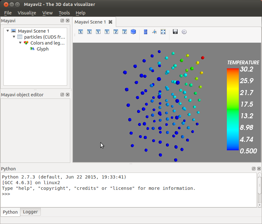
Use the provided example to load data from a SimPhoNy engine and visualise directly in Mayavi2.

In the Mayavi2 embedded python interpreter, the user can access the SimPhoNy engine wrapper associated with the EngineSource via its engine attribute:

# Retrieve the EngineSource
source = engine.scenes[0].children[0]

# The SimPhoNy engine wrapper originally defined
source.engine

# Run the engine
source.engine.run()

# update the visualisation
source.update()